


 2022-10-19
in
2022-10-19
in

 14 min read
It started simply enough. I had a hard disk failure, an SSD ironically, which forced me to start rethinking how I was managing my storage. I decided to buy one giant 16 TB USB 3.0 spinning disk to add as a giant drive and leave the high speed internal SSDs for things like the host OS, development VMs, etc. The immediate question was if I should format it as one big partition or not. I thought it was a simple question but ironically there was a dearth of modern articles really exploring the question versus the how to do it. Does it matter or does the OS make it irrelevant? That’s a complicated answer but I have some data to help me make a decision on the matter that I’m going to share here.
Standard Benchmark: More Questions than Answers
Fortunately for me the GNOME desktop ships with a standard disk utility called UDisks . Along with being able to partition and format disks it also has support for doing diagnostics and benchmarks. So I figured I’d just run a quick benchmark to see how this USB 3.0 spinning disk would perform. I’m not expecting the fastest disk in the world since it is a budget physical hard disk but it would still be curious to see what was what. So after formatting the whole 16 TB to ext4 this is what I got
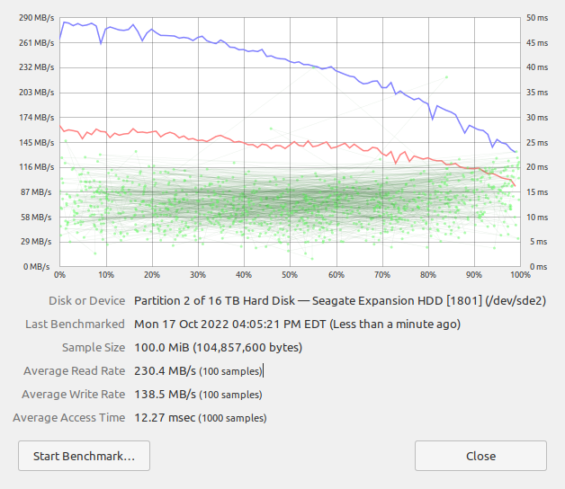
Full disk benchmark showing degradation over test
Things started off great, with average read rates pushing 300 MB/s and write rates of 160 MB/s or so. But as the test went on and on the results got worse and worse, ending at less than 140 MB/s read and about 90 MB/s write. The read rate dropped off much faster than the write rate but both have noticeable performance differences. This made me have even more questions than when I started. Is this just a test artifact? Is this a performance problem because of the physical geometry of the disk? Is this a performance problem because of the caching? The only way to start answering these questions is to start interrogating the hardware more deliberately.
Testing Physical Geometry Hypothesis
In the olden days it was considered a necessity to partition hard disks for performance reasons. Most of that was around the fact that you needed larger sectors for the larger drives so lots of smaller files would end up wasting space. While that is still 100% true it matters a lot less today than it did decades ago. There was always the debate about performance advantages as well. The question again for today was is any of that practically true today. Obviously over the above benchmark things degraded more and more. Is that a geometry problem or is something else going on? I believe it is a physical geometry problem that is creating this performance change. To test that I partitioned the drive into eight equal 2 TB partitions and re-ran the benchmark suites on each partition. If the problem is geometry related then it should have a comparable curve to the one giant partition test. If the problem is one of above a certain size there is a degradation of performance than I should see relatively uniform and comparable curves for each partition.
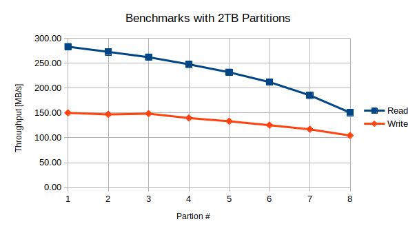
Summary of Benchmarks run on sequential 2 TB partitions
As we can see the numbers and trends are generally true but not completely identical. We start off with essentially the same read and write performance but the apparent read performance starts dropping off a bit faster. When we get to the end we essentially get down to the same levels however. For example here are the charts for the first and last 2 TB partitions:
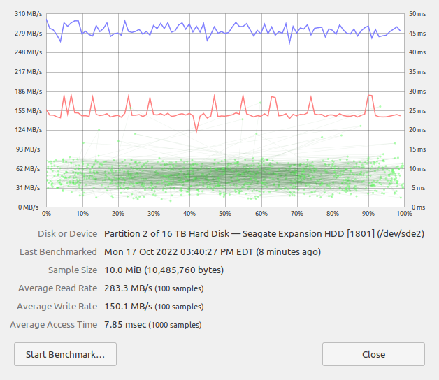
First 2TB Partition Detailed Benchmark
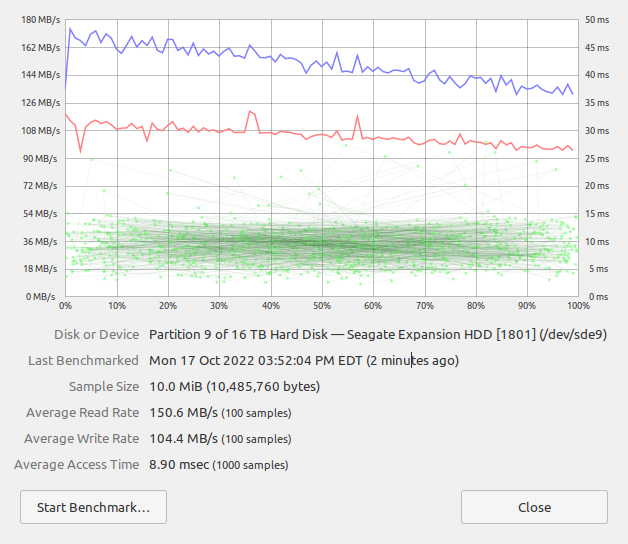
Final 2TB Partition Detailed Benchmark
It is clear that the performance curves are very comparable to what we saw for the respective beginning and end of the one large disk partition benchmark case. We are therefore dealing primarily with a disk geometry generated performance artifact not something inherent in the benchmark, caches, or partition size irrespective of location on the disk.
What happens if we take this to an extreme of having a small, 256MB partition at the front of the disk and another small 256 MB partition at the back? The smaller sizes do give us some additional performance on each side but we can still see a performance degradation. The front partition averages 383 MB/s read and 155 MB/s write performance. The back partitino averages 213 MB/s read and 102 MB/s write. Again, both of these are better than their corresponding 2TB front/back tests. So there is some benefit to smaller partitions from that perspective but nothing compared to relative location of the data on the platter.
One thing of note which I haven’t listed here is the dramatic difference in average access times for the different sizes. When the partition size is 256 MB that number is 2.5 ms for the front of the disk and 2.7 ms for the back. With the 2 TB partitions that number varies from 7.9 ms for the front and 8.9 ms for the back. The number for the full disk all at once, as you see above, is over 12 ms. This will have performance implications for accessing lots of small files.
From all of this we see the write performance differential is almost a factor of 2 and the write performance is about a factor of 1.5. The differential in access times for the larger to smaller (practical) partitions is comparable to this different in write performance. These are therefore not insignificant or marginal performance differences. At least it is not in this benchmark. What does this look like for real world performance?
Real World Loading Test
With the benchmarks showing pretty significant performance differences from one area of the disk to another the next question is if that holds up in real world usage and is it something that would show up immediately as noise in the performance or over time as the drive fills up. To test this I created two short Dart programs that would allow me to fill up the hard disk systematically and to read from it in order to get benchmarks of both sides. The tools described below can be found in this GitLab repository
Write Testing
In order to determine how write performance changes over the course of the disk filling up the program allows me to specify the total amount of disk allocations to create, the size of each of the files, and some other parameters. In order to make sure the operating system isn’t getting too clever with caching etc. the files themselves are always randomly generated bytes for the requested size. Originally this was all written in Dart. While disk write performance was pretty solid the overhead of the memory allocations and/or randomizations was making the run times several times longer than the write operations themselves. In order to ensure as timely an execution as possible the Dart program now calls out to the command line tool dd with the input being /dev/urandom as the source. This is as efficient as possible. The files themselves are named with the iteration number in them to allow reconstruction of estimating where in the filling operation it falls.
When this program is executed for this test it was setup to write out a series of 1 GB sized files until the entire drive was completely filled. For each write we measure the wall clock time in microseconds it took for the dd command to complete, how many bytes were written in that iteration (which is constant in this case) and how many bytes total. From this we can clearly graph where relative to the front of the disk usage percentage this file is allocated and the throughput for the operation.
Read Testing
While we were able to use an operating system tool rather than pure Dart to write the files out, we stuck with using a pure Dart program for the read test. The core of the read test simply uses Dart’s synchronous File.readAsBytesSync method to read the entire file from the disk into memory and then to calculate the total bytes. This is a pretty minimal overhead operation. The program has some logic so that it can parse the filename to figure out where on the filling process the file was created.
While the write test had no choice but to linearly fill the entire disk in order to measure write performance as the drive fills up, in the case of the read tests we can sub-sample the files themselves. The program can be run in a mode where you specify a specific number of files to sample. It will then sample the entire set spanning across all of the files. For example, if you specify three samples you’d get the first file, the last file, and a file in the middle. If one runs the program in “shuffle” mode then it selects files at random across the entire set rather than linearly.
In order to ensure that we aren’t dealing with cached files it is important to run this test on a freshly booted system. The caching behaviors themselves will only be apparant for smaller runs. For example a linear run that samples the 1st, last, and middle files of specific indices accessed those files in a way where a second run will produce a cache hit. The first time through the throughput was between 197 and 247 MB/s. That’s consistent with the throughput we measured in the benchmarks. However the throughput on the second run where all of these files are now in caches produces throughput rates of 2066 to 5344 MB/s. Obviously if we are benchmarking the disk we want to minimize the chance of having noisier data from cache hits.
Real World Results
Let’s start by looking at the write tests performance. In the below graph we see the throughput for each of the over 1GB files that were written to the full disk. Files written while the disk was empty are on the left side of the graph and so on until the disk is full. The magnitude of the curve is higher than the benchmarks by quite a bit. I believe this is because we are writing large files instead of small ones, which it can do more efficiently. While it starts at a higher magnitude the general trend is similar, albeit a bit more exaggerated even. While we start off bouncing around 250 MB/s until we get about 25% full it starts a slow and then faster decline down to about 98% full. It is at that point that for some reason the write performance recovers back to the same level as near the 0% case. Is that a sign that the drive was reserving the last few percent near the same physical location as the start of the disk? Is it some other artifact? It is very difficult to say either way from here.
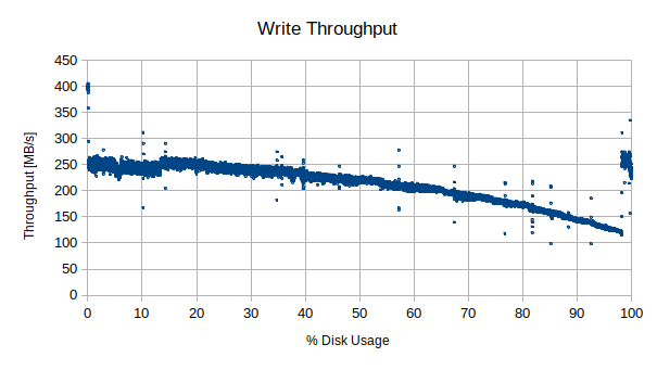
Write throughput over entire disk
Below is a chart of the read results for 1000 of the generated files. As stated above, because each file is tagged with the sequence with which it is written we can estimate where in the fill process the file was created so at which stage of filling the disk. Assuming that aliases to some consistent geometric fill with the disk it would then correlate performance wise with the writes too, just as in the benchmark. The test was run in two different ways. The first run of the test marched through the files linearly with equal spacing to span the entire disk with 1000 samples. The second run 1000 files were randomly sampled from all over the disk. The computer was rebooted between runs to make sure the caches had been flushed.
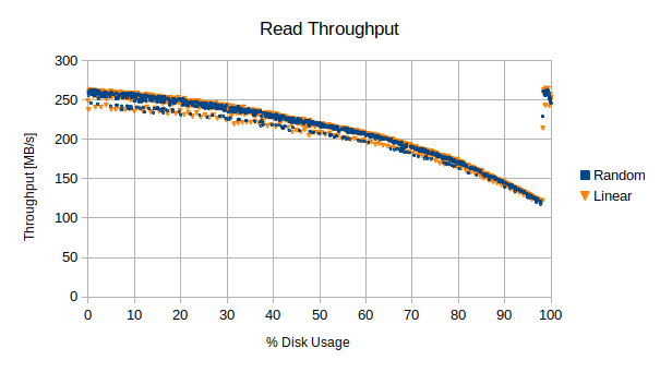
Read throughput over entire disk
In this particular case we can see that we started off with a read speed that wasn’t as high as in the benchmark. However it is in the same comparable area. The drop off also didn’t go down as low as it did in the benchmark. It was trending in that direction but like with the write performance measurements, once we cross the 98% full mark the performance recovers back up to the same values as near the beginning of the disk. The overall performance differential is on the same order and overall shape as the benchmark except for that step up at the end.
Conclusions
One big conclusion from all of this is that the benchmarks do act as reasonable proxies for the disk throughput, including simulating the performance changes as the drive fills up. This is probably the most optimal performance as the drive fills up though since there is no fragmentation. The level of fragmentation is going to be very operating system dependent. Also file system tricks that may be used to reduce fragmentation could see the performance degrading faster in real world conditions.
The second big conclusion is that there are serious differences in read and write performance over the span of the disk, with or without partitioning. Data access near “the front” of the disk are going to be 1.5 to 2 times faster than those on the back of the disk. That appears to be both for the case of one enormous disk partition or it being divided up. It seems to be entirely driven by physical geometry. The average access time however is driven far lower via partitioning. With the full disk being over 12 ms and a 2 TB partition, so 1/8th of the disk, down to 9 ms, there potentially be performance impacts from this that could be addressed by partitioning.
The third big conclusion is that if you have storage throughput requirements that are above the minimum threshold these levels indicate then you may want to seriously consider partitioning the drive to isolate the higher performance applications to the faster parts of the drive. If all you are doing is using this for backups, longer term storage, and relatively small file retrieval then it probably won’t matter. That gets back to the practical versus theoretical performance reasons for partitioning the drive.
If I were so inclined I’d recommend repeating the test both uniformly with much smaller file sizes, perhaps 1 MB, and then again with irregular sizes and create/delete operations etc. I also would be interested in exploring what is happening in the post-98% full region as well. Those are out of the scope of what I was trying to do which was determine if I should be treating this as one enormous image or not. So while I find those areas of study interesting I will not be doing that myself for the foreseeable future.
My Partitioning Scheme from this Research
After all of that I have decided to partition my drive after all. While most of this drive is going to be used for storage of lots of files that will get accessed infrequently there are some aspects of usage that will benefit, but not require, higher performance. I use lots of virtual machines for my development. For ones that are used less frequently I store them on secondary drives. When they have been offloaded to physical disks they can feel sluggish. Those existing physical disks however are slower than this drive even though they are attached via drives even though they are connected directly not over USB. This new drive exceeds those older drives for most of the performance curve. However if creating a smaller partition in the front could dramatically improve that performance (hypothetically giving me just half the throughput of these older NVMe drives but unfortunately with much larger access times) then it is worth doing.
I also have requirements to be able to use this drive for transferring files between Macs and Windows machines as well as my Linux box. I could use MacFUSE for doing this with ext4 but it seems like it’d be better to have an ExFAT partition for that work. I also want to use this partially for doing a full backup of my primary disk to this external drive. That drive is 2 TB itself and I want to make room for snapshots. I therefore envision a configuration as as follows:
- Partition 1 (1st 2 TB) for higher performance applications: This should give me both read and write performance on larger files of upwards of 250 MB/sec which again is half of this machine’s NVMe drives.
- Partition 2 (Next 9 TB) for bulk storage: these are long term photos, videos, office documents, zipped up archives of my various software experiments, etc. Based on the curves we should still get performance above 200 MB/s on reading files and 140 MB/s up to 220 MB/s writing.
- Partition 3 (Next 3 TB) primary drive local backup. This will be the first partition in the more degraded performance area but for backups this shouldn’t be a problem
- Partition 4 (Last 2 TB) ExFAT transfer partition: This is going to be the slowest partition but since it is only going to be used for transfers between machines periodically I don’t care.